Chapter 2

2. Some models from business economics

Nonlinear functions are useful in modelling different phenomena. Here some models from business economics are presented and the theory of dynamical systems is applied to analyze their dynamics.

2.1. An investment model

Cubic functions of the form , (l > 1), have been considered useful in approximation of investment functions [Puu89]. The function f_l (x) has a local maximum and a minimum around zero and these can be considered as the "floor" and "ceiling" for the investments. Investments I_t at time t may be approximated by:

(2.1)

where the income at time t-1 is denoted by Y_t-1. l is used as an adjustment parameter.

Figure 9. The cubic function

From the equation f_l (x)=x the following fixed points can be found:

and their stability can be determined by calculating | f_l’(x_i*) |, for i=1,2,3.

The fixed points x₁* and x₃* are attracting for 1<l <2 and repelling when l >2. The fixed point x₂*=0 is repelling for all l >1. When l =2 a period-doubling occurs, which can be verified with its theorem, proof. The bifurcation diagram is shown in figure 10.

Figure 10. The bifurcation diagram for f_l (x),

The figure shows that f_l is chaotic when l =3, proof.

2.2. A model for capital investments

Capital investments of a firm is denoted by g_t. A standard exponential growth model can be written as:

	g_t=(1+k) g_t-1
	=(1+k)^t g₀	(2.2)

where g₀ is the initial level of capital investments. The growth rate (which is assumed to be positive) is denoted by k. A modified model is used (for estimation of the internal rate of return) in [Sal97] where periodicity is included with a sinus term as:

(2.3)

where A and C are the amplitude and the length of the business cycle. f is used for adjustment of the cycle. The model (2.3) can also be recognized as a solution to a second degree difference equation, proof.

The difference equation with the solution (2.3) can be written as (proof):

(2.4)

The models (2.2) and (2.3) has 0 as the only (repelling) fixed point. These models are useful in modelling growing trends, with or without cycles [Sal97].

Figure 11. The investment models g_t and g_t^P.

2.3. An advertising model

An interesting chaos-analytic study of a nonlinear advertising policy can be found in [Luh97]. The changes in Goodwill g(t) are modelled as a function of the advertising outlay a(t), as the following:

(2.5)

where r is the depreciation rate of the Goodwill. The model (2.5) can be written (with inclusion of a lag-term) in discretized form as:

g_t+1 = g_t - rg_t + a(t-t )

(2.6)

The model (2.6) describes that the change of goodwill depends on the amount of advertising a certain time, t, ago (t is here a natural number). If t=1 (2.6) describes a twodimensional dynamical system.

The effect advertising is modelled linearly, nonlinearly and bounded as the following:

Linear marketresponsmodel:

g_t+1 = g_t - rg_t + a(g_t-t)

(2.7)

Nonlinear model:

g_t+1 = g_t - rg^q_t + a(g_t-t)

(2.8)

Bounded model:

g_t+1 = g_t - rg_t + a(g_t)

(2.9)

The following advertising function is used in the above models:

a(g_t) = bg_te^{1/s(1-g^s_t)}

(2.10)

The parameters b and s are used for scaling of the function a(g_t ). In [Luh97] fixed points (of the above models) are calulated and periodical points are described by bifurcation diagrams. Parametervalues when the models are chaotic are also identified using Lyapunov exponents.

Consider (2.7) with t=1 :

g_t+1 = (1-r)g_t+bg_t-1e^{1/s(1-(g_t-1)^s)}

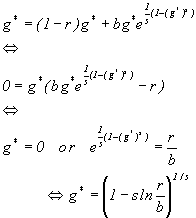
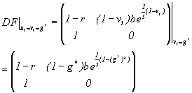
The fixed point g* may now be calculated:

The model may be substituted as:

The Jacobimatrix evaluated in g^* is then:

The eigenvalues may now be calculated:

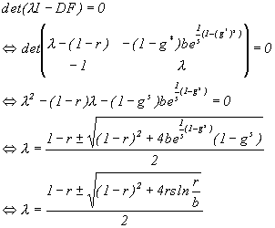
The behavior of the fixed point above may now be determined with the parameter values (b, r and s).

Contents | Chapter 1 | Applications